This tutorial
will take you through the steps required to set up a cancer
classification example in the NeuroShell® Classifier. The data in this
example is located in a file called CANCER.CSV that is located in the
Examples subdirectory of the directory where the NeuroShell® Classifier
is installed. This directory is usually C:\NEUROSHELL
SERIES\CLASSIFIER, which is the default directory that is created when
you install the program.
Cancer
Classification
Imagine that your company, Diagnostic Services, wants to develop
a neural network model that determines whether a patient has skin
cancer without performing a biopsy.
NOTE: This is not a real medical
application. It should be used for instructional purposes
only. The number of patient records and the input values are
not sufficient to build a clinically acceptable diagnostic
assistant.
Since you are new to using neural
networks, you use the Instructor in the NeuroShell® Classifier.
Instructor Steps 1 and 2 - Begin the Program
You
create a data file that include
s information about 50 patients. This
file is a comma separated text file, since your Windows Control Panel is
set to U.S. number formats and
list separator
. The Instructor begins by prompting you to load a data file.
Instructor Step 3 - Select a Data File
A dialog box is
displayed which allows you to select the CANCER.CSV file in the
C:\NeuroShell Series\Classifier\Examples subdirectory. (The
subdirectory may be different if you chose to install the NeuroShell®
Classifier in a directory other than the default.) Push the next button
to view the spreadsheet.

Instructor Step 4 - The Data File
The spreadsheet
is displayed in the NeuroShell® Classifier datagrid.
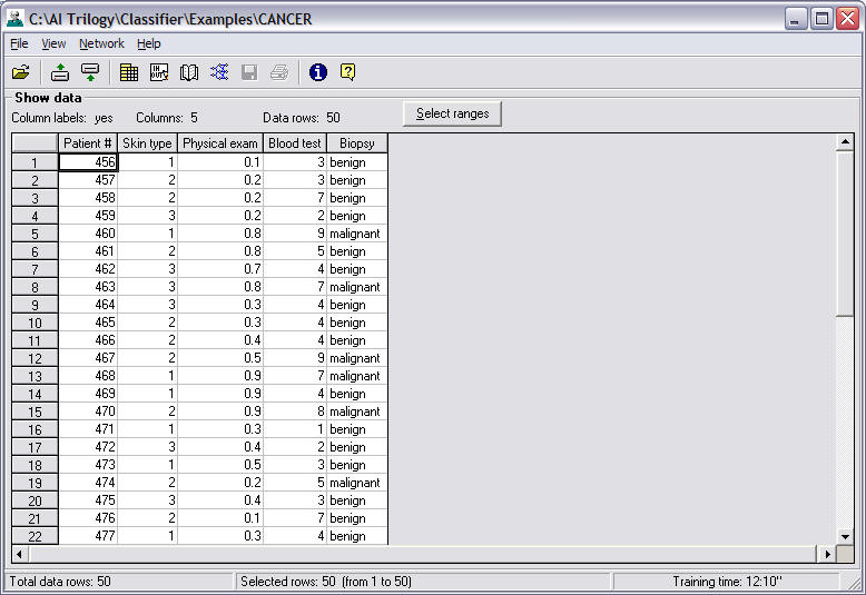
The top of the datagrid displays some information
that is useful in determining if you opened the correct file.
The path name of the file shows the location of
the file on the computer’s
hard drive, including the drive letter (C), the directory and
subdirectory if there is one, and the name of the file. The
screen also shows if the file include
d column names by placing a
yes or no in the initial label row detected box. The number of
columns and rows in the file are also displayed.
Note that column names are at the top of the
datagrid and the data rows are numbered. Note that each
patient's
data is include
d in a row
in the datagrid. The
input variables that affect
the classification of cancer are
columns
in the
datagrid.
Input values:
Patient #: A
control number assigned to each patient.
Skin Type: Values
ranging from 1 to 3 that describe skin color: 1 = fair, 2 =
medium, and 3 = dark.
Physical Exam:
Values ranging from 0 to 1 which represent a probability value
that a patient has skin cancer. An examining physician assigns
the values to each patient.
Blood Test: Values
ranging from 0 to 10 that represent a reading from a blood test
that looks for cancer cells.
The output you are trying to predict is the
column labeled biopsy. For the training data, the diagnosis of
malignant or benign was confirmed by biopsy. Your model will be
an attempt to make the correct diagnosis without the patient
having a biopsy.
Instructor Step 4 allows you to load a trained
neural network if you have already created one by pushing the Existing
Network button. Since this is the first time you are creating
this model, push the next button.
Instructor Step 5 - Select Rows for Training the Model
The Instructor allows you to choose some rows
from your data file that will be used to train the neural network. You
may use the rows that are not chosen (an out of sample set) to
test the neural network to see how well it is performing after it has
been trained.
Since this is a relatively small data file with
only 50 rows of data, you decide to train the neural network using all 50
patients. This is the default so you do not have to do
anything.
If you had wanted to select some rows for
training and other rows for an out-of-sample set, click on the
Select ranges button.
Push the Next button to jump to Instructor Step
6.
Instructor Step 6- Decide How to Train the Model
This step of
the instructor begins a series of steps that involve a single screen in
the NeuroShell® Classifier. The purpose of the screen is to:
1. Select the
input variables and the predicted output.
2. Select the
training strategy.
3. Select the
graphic screen that will be displayed while the neural network is training.
Select
the Input Variables and the Predicted Output
Note that
the column names from your data file are displayed in the two
list boxes on the left side of the screen.
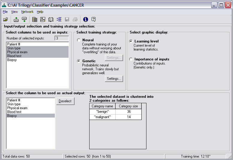
Select the inputs from the top list box. Use the
left mouse button to click on Skin type, then strike the shift
key and then click on Blood test. All of the column names
between the two are automatically selected.
If you had wanted to pick some columns and then
skip others, you could have hit the control key and then clicked
on individual column names.
Next, in the bottom list box click on the column
Biopsy, which is the column in your data file that contains the
classification for each set of inputs. The NeuroShell®
Classifier can only have one output column for each problem.
Note: If a column is selected as an input, it may not be
selected as an output. If a column is selected as an output,
the program will not allow you to select the same column as an
input.
If you didn't make any selections, the program
assumes that the last column is the output and all other columns
are input variables.
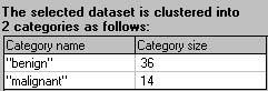
Dataset Clusters
The screen
displays a list of each category in the output column and the
total number of examples or rows that occur in each category.
You can use this summary to determine if your training data is
"balanced" with a similar number of examples in each of the
output categories. If the categories are unbalanced, you
may want to consider using a different genetic optimization
goal.
Instructor Step 7 - Select a Training Strategy
Notice that the screen offers two different types
of training strategies. Since you are learning how to use the
program, you decide to train the neural network both ways.
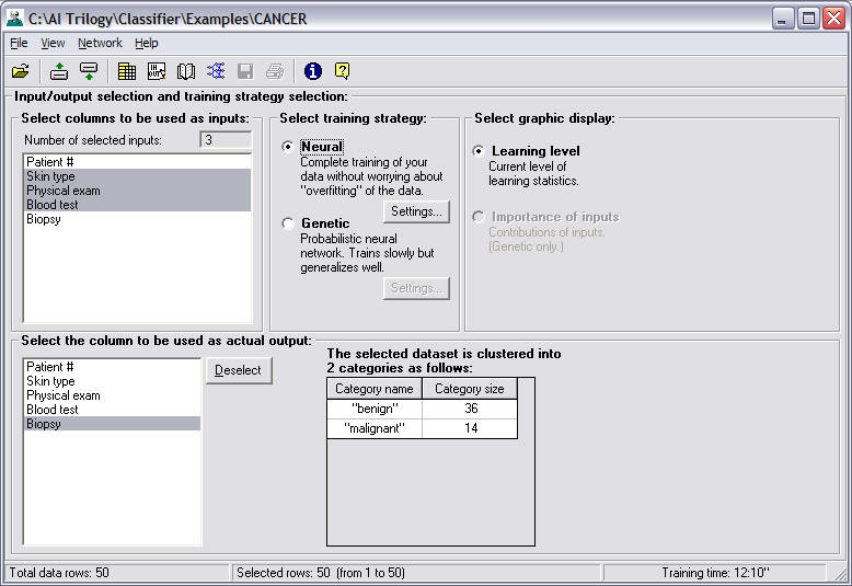
First choose the Neural Training
Strategy, which uses a neural network that dynamically grows hidden neurons
to build a model which generalizes well. It trains fast.
Push the Next button to select a graphic
display. (You'll get a chance to select the Genetic Training
Strategy later in the Instructor.)
Instructor Step 8 - Select a Graphic Display
Next choose which graph will be displayed
while the neural network is learning.
For the Neural Training Strategy, your
option is:
Learning Level
This option graphs the percent of correct
classifications against an increasing number of hidden neurons as they
are added to the neural network.
Push the Next button to begin training
the neural network.
Instructor Step 9 - Train the Model
Notice that the green light is on while
the neural network is training and the graph you selected is displayed on the
screen. The red light is displayed when training is complete.
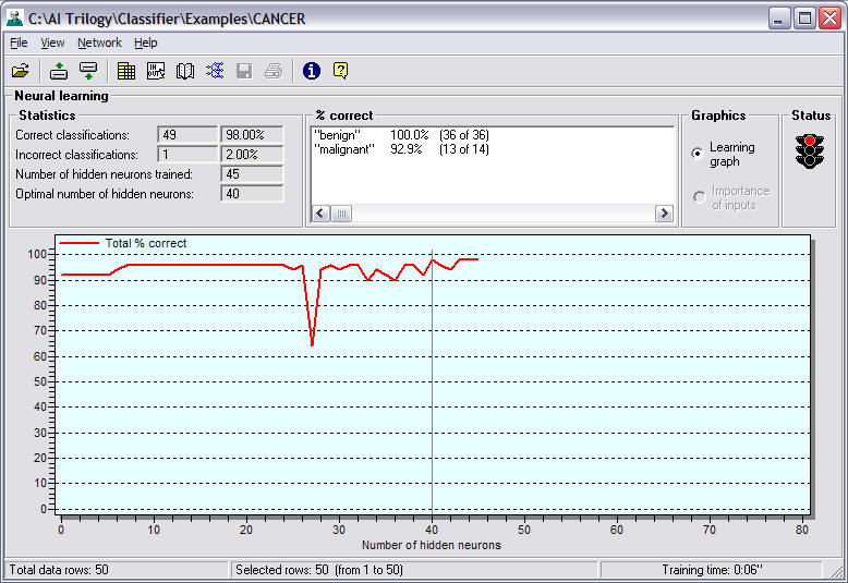
Several statistics record the neural network’s
progress:
Correct classifications:
Displays the
total number
and
percentage
of examples (rows) in the training data that the neural network
categorizes accurately. The neural network does this by comparing its
classification with the category specified for each example in
the training data and then summarizing the results for the
entire training set.
Incorrect classifications:
Displays the
total number
and
percentage
of examples (rows) in the training data that the neural network
categorizes inaccurately. The neural network does this by comparing
its classification with the category specified for each example
in the training data and then summarizing the results for the
entire training set.
Number of hidden neurons trained:
Displays the total number of hidden
neurons that have been added while the neural network is learning.
Training
the
neural network involves adding hidden neurons until the neural network is able to make
good classifications.
Optimal number of hidden neurons:
Displays the number
of hidden neurons that best solves the classification problem.
%
correct:
Displays the total number and percentage correct for each
possible output category. Click on the arrows at the bottom of
the box to display the entire text.
The Correct Classifications by Hidden Neuron
graph shows the number of hidden neurons graphed against the
percentage of correct classifications.
Click on the right mouse button when the pointer
is inside the graph to display options to export or print the
graph for use in another document.
Status
Green light:
neural network is continuing to learn the training data.
Red light: neural network
has finished learning the training data.
Push the Next button to apply the neural network to the
training data.
Instructor Step 10 - Obtain Results
This step of
the Instructor displays a variety of statistics and graphs to explain
the neural network's results. For this example, the trained neural network is
applied to the 50 data rows used to train the neural network. If,
however, you had selected different rows for training and applying the
neural network in Instructor Step 5 - Select Rows for Training the Model, a
different number of rows would be processed on this screen. The
probabilities shown are in U.S. number format since that is how your
Windows Control Panel is set.
Enhanced generalization (for noisy data):
Click in the check
box to turn this option on or off.
Enhanced Generalization should not be used unless
your data is "noisy", i.e., it is not a smooth function of the
input data. Enhanced Generalization is a different method of
applying the neural network that tends to smooth out the classification
for out-of-sample data. When turned off, the neural network will give
better results for data in the training set. When turned on,
the neural network will give better results for data not include
d in the
training set (out-of-sample data) if the data is noisy. The
difference in results is often more noticeable when the Neural
Training Strategy is selected rather than the Genetic Training
Strategy. In some instances when the Genetic Training Strategy
is selected, you will not notice any effect from Enhanced
Generalization. If you train with the Genetic Training
Strategy, then apply the neural network to the
training
data with Enhanced Generalization off, the neural network may do even
better than it did during training.
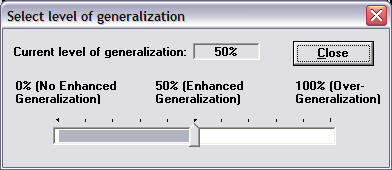
Advanced Generalization (Neural Training Strategy only):
Pressing the Advanced Button will allow you to select the level
of generalization from 0% (No Enhanced Generalization) to 100%
(Over Generalization). A setting of 50% is equivalent to
Enhanced Generalization. The default value, when the Enhanced
Generalization button is checked is 50%. We recommend that you
apply a trained neural network to a test set of data which you already
know the actual value and adjust the level of generalization
until you achieve desired results. Use the same setting when
applying to out of sample data.
Note that
you do not have to retrain the neural network in order to turn
Enhanced Generalization off and on. The neural network is
automatically applied each time the condition of the
check box is changed.
When you
save a neural network, the program will remember what level of
generalization you had previously set.
Rows processed:
Displays the
number of data rows
that were analyzed by the neural network in order to make a
classification.
Rows classified correctly:
Displays the
total
number and
percentage
of examples (rows) in the file to which the neural network is
applied that the neural network categorizes accurately. The
neural network does this by comparing its classification with
the category specified for each example in the data file
and then summarizing the results for the entire data
set. If there are no actual values in the data file,
the term N/A for non-applicable appears in the total
number and percentage boxes.
Rows classified incorrectly:
Displays the
total number and
percentage
of examples (rows) in the file to which
the neural network is applied that the neural network categorizes
inaccurately. The neural network does this by comparing its
classification with the category specified for each
example in the data file and then summarizing the
results for the entire data set. If there are no actual
values in the data file, the term N/A for non-applicable
appears in the total number and percentage boxes.
Rows not classified:
Displays the
number of rows the neural network was unable to analyze. This
situation only occurs when the Genetic Training
Strategy is used and the
neural network is being asked to classify an example that is
very dissimilar from the training data
.
Actual and predicted outputs:
Display option:
Allows you to change the rows that are displayed
in the Actual and Predicted Outputs box. Click
on the arrow to select
All Rows:
Displays results for every row in the data file
to which the neural network was applied.
Only rows not classified:
Displays results for the rows in the data file
to which the neural network was applied that the neural network
was unable to analyze.
Only correct classifications:
Displays results for the rows in
the data file to which the neural network was applied that
the neural network placed in the correct category.
Only incorrect classifications:
Displays results for the rows in
the data file to which the neural network was applied that
the neural network placed in the incorrect category.
Display box: Displays a scroll
box which lists the:
Row #:
The number of the row in the data file for each
example. An asterisk is displayed beside the
row number when the model makes an incorrect
classification.
Actual:
Displays the category classification as it
appears in the data file.
If
NA appears in the Actuals column, it means that
the neural network was applied to a file that did not
contain actual output values. This usually
occurs when the trained neural network is applied to a new
data file for which the predicted outcome is
unknown. In this case, only the neural network’s
classifications will be displayed in the
Predictions column.
Classified as:
Displays the category classification predicted
by the neural network.
If
NA appears in the Predictions column and the
Genetic Training Strategy was used, it means
that the neural network was applied to a set of input
values that are quite different from the
examples used to train the neural network. The
solution is to include
representative examples
of any type of classification in the training
data. In this example you need to include
a
variety of sets of input values that could
result in either a benign or malignant
classification.
Precision - Full or Reduced:
Changes the number of decimal places displayed
for the neural network's classifications.
Output
categories and strengths: Displays a
column for every possible classification
category and the neural network's classification value
for each category. When the neural
training strategy is selected, this value is the
neuron activation strength for each category
based on that set of input values. This
value can loosely be though of as a probability.
When the genetic training strategy is selected,
this value is the probability that set of inputs
should be include
d in the designated category.
For both the neural and genetic training
strategy, the values for all categories add up
to 1. When the value is close to 1 in a
category, the neural network is more confident that the
example set of inputs belongs to that particular
category.
Click on the
arrows to scroll left and right and up and down
on the box to display all data.
Type of
Statistics
When the trained
neural network is applied to data, one of three types
of graphics may be displayed by clicking on the
corresponding button. You can change the
graph simply by clicking on another button.
Note: If
your file does not contain actual output values,
the Agreement Matrix and ROC Curve graph are not
available for selection because they are created
by comparing actual with predicted values.
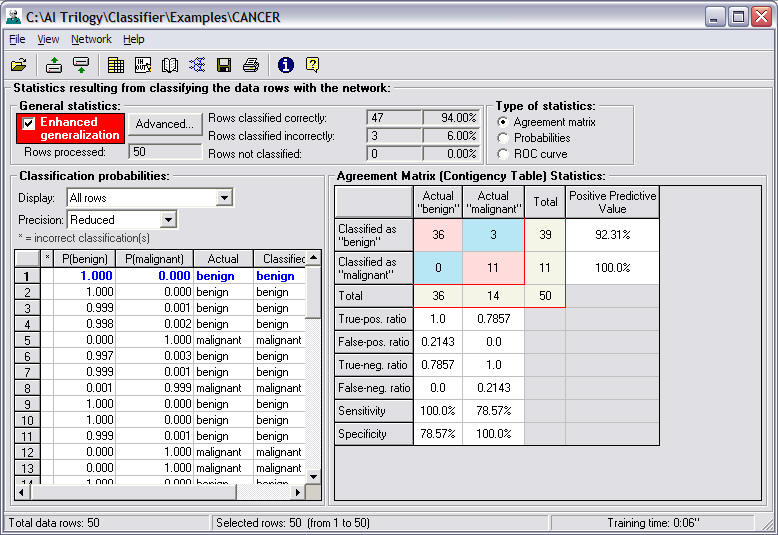
Agreement
Matrix (Contingency Table):
The agreement
matrix shows how the neural network's
classifications compare to the actual
diagnosis in the data file to which you
apply the neural network. The number of
examples from the data file that match the
comparison criteria is displayed in the
appropriate columns and rows.
The column
labels Actual benign and Actual
malignant refer to the category
classification in the data file.
The row
labels Classified as benign and
Classified as malignant refer to the
neural network's predictions.
In this
example, when the neural network was applied to 50
rows of training data, there were 36 actual
examples of patients without skin cancer
classified as benign, which the neural network
confirmed. There were 14 actual
example of patients with skin cancer
diagnosed as malignant, but the neural network
classified 3 of those examples as benign and
11 as malignant.
True-pos. ratio
(True-Positive Ratio, also known as
Sensitivity)
is equal to the number of
patients classified as malignant by the
neural network that were confirmed to be
malignant through biopsy, divided by the
total number of malignant patients as
confirmed through a biopsy. It is also
equal to one minus the False-Negative
ratio.
False-pos. ratio
(False-Positive Ratio)
is equal to the number of patients
classified as malignant by the neural network
that were confirmed to be benign through
biopsy, divided by the total number of
benign patients as confirmed through a
biopsy. It is also equal to one minus
the True-Negative ratio.
True-neg. ratio
(True-Negative Ratio also known as
Specificity)
is equal to the number of patients
classified as benign by the neural network that
were confirmed to be benign through
biopsy, divided by the total number of
benign patients as confirmed through a
biopsy. It is also equal to one minus
the False-Positive ratio.
False-neg ratio
(False-Negative Ratio)
is equal to the number of patients
classified as benign by the neural network that
were confirmed to be malignant through
biopsy, divided by the total number of
malignant patients as confirmed through
a biopsy. It is also equal to one minus
the True-Positive ratio.
Sensitivity and Specificity
The terms sensitivity and
specificity come from medical
literature, but are now being used for
other types of classification problems.
In this example, sensitivity and
specificity are calculated by comparing
the neural network's results with the biopsy
results in the 50 rows of training data
for all possible output categories
(benign and malignant).
When you examine the column
labeled "Actual
malignant":
Sensitivity (true positives)
equals the number of patients the
neural network classifies as malignant that are
also confirmed as malignant by biopsy
(11) divided by the total number of
patients confirmed as malignant by
biopsy (14). 11/14 = .7857 or 78.57%,
the sensitivity of the model for
malignancy. Sensitivity can be
thought of as the probability that the
model will detect the condition when it
is present.
Sensitivity (true
positives) equals 1 minus the number of
false negatives.
Specificity (true negatives)
equals the number of patients the
neural network classifies as benign that are
also confirmed as benign by biopsy (36)
divided by the total number of patients
confirmed as benign by biopsy (36).
36/36 = 1 or 100%, the specificity of
the model for malignancy.
Specificity can be
thought of as the probability that the
neural network model will detect the absence of
the condition. Specificity (true
negatives) equals 1 minus the number of
false positives.
When the category is benign,
the terms are reversed.
Probabilities
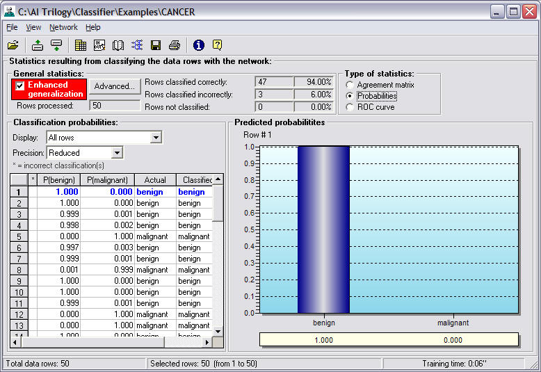
The probabilities graph displays the
neural network's prediction for each selected row
in a bar chart. A separate bar chart is
displayed for each row and the appropriate
row number is displayed at the bottom of the
chart. The bar chart depicts the chance the
set of inputs in that row will lead to a
classification in each of the output
categories. The probability values for all
output categories add up to 1.
One reason to use this
graph is to examine incorrectly classified
rows. If you have two output categories and
the probabilities are fairly close, with
values such as .49 and .51, you'll know that
the neural network did not have enough information
to make an unequivocal classification. You
may need to add additional inputs to the
neural network to help it discriminate better. If
the example was incorrectly classified and
the probabilities are far apart, with values
such as 0.904 and 0.096, you may want to
make sure the input values and the actual
output are correct.
ROC Curve
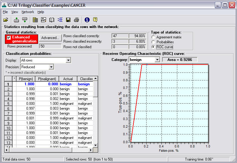
The ROC (Receiver Operating
Characteristic or Relative Operating
Characteristic) Curve graphs the
false-positive ratio on the x axis and the
true-positive ratio on the y axis for the
category selected in the Category box that
is displayed above the curve. A yellow
marker is plotted on the curve to show the
intersection of the True-positive and
False-positive values of the neural network
classifications for the selected category.
In other words, the yellow marker on the ROC
curve corresponds to a point where the
NeuroShell® Classifier, with your trained
neural network, converts continuous probabilities to
binary classifications. Click on the arrow
in the Category box to select a different
category.
The area under the curve
represents how well the neural network is
performing. A value close to 1 means that
the neural network is discriminating very well
between the different output categories. For
this example, it means that the neural network
classified malignant examples as malignant
and classified benign examples as benign. A
value of 0 means that the neural network is a
perfect inverse classifier, which means that
all examples which should be classified as
malignant are classified as benign, and all
examples which should be classified as
benign are classified as malignant. For more
information about ROC curves, refer to the
Swets paper in the References section.
NOTE: When your model has
two classes and you want to change the
position of your classifications on the ROC
curve, you would have to change the
threshold of classification to something
other than the .5 the Classifier uses.
Save Classifications
You decide you want to save a copy of the
neural network’s classifications in a file so you can
compare these answers with those from the
Genetic Training Strategy neural network that you will
train later. Click on the diskette icon on the
toolbar or go to the File Menu and select Save
classifications on disk. A file is created that
include
s the columns and rows from the original
file plus an additional column of neural network
classifications. The file is called CANCER.OUT.
The first part of the name comes from the data
file used to train the neural network, and the program
adds the .OUT extension. The file name may be
changed in the dialog box. This file is a comma
separated file that may be read by spreadsheets,
notepads, and word processors. The .OUT file is
written to match the file format of the input
training file with regard to list separator and
decimal symbol .
Print Classifications
For quick reference, you click on the printer
icon on the toolbar that prints out a report on
the default printer attached to your computer.
The report include
s the row number, an actual
output value from the training data, and the
corresponding neural network classification for each
row. You may also select the File Menu, Print
classifications option.
Push the Next button to jump
to Instructor Step 11.
Instructor Step 11 - Apply the Model to the Remaining Data Rows
If you had not used all of your
data to train the neural network, you could use this step of the Instructor to
select the remaining data rows and apply the neural network to obtain results.
Select the remaining rows by
using the Select Ranges button. Once you select the rows for testing
the neural network, push the Back button to return to the previous screen where
the results of applying the neural network to the remaining data rows will be
shown.
Since you have already used all
of your data, push the Next button to jump to Instructor Step 12.
Instructor Step 12 - Save a Copy of the Neural Network
Use this step of the Instructor
to save a copy of the neural network on disk for later use. You would not want
to train the neural network over again to use it later.
Save the neural network by pushing the Save
Net button. The neural network is saved under the default name of CANCER.NET. The
dialog box that is displayed gives you an option to change this name and
directory location. Record the name of the file so you can find it
later. Also record the neural network type, which is neural.
Push the Next button for
information on retraining the neural network.
Instructor Step 13 - Retrain the Neural Network
Since you are learning how to
use the NeuroShell® Classifier, you decide to retrain the problem with
the Genetic Training Strategy for comparison purposes. Push the Retrain
Net button, which takes you back to Step 6 of the Instructor.
Instructor Step 6 - Select Inputs/Outputs (Genetic)
This part of the Instructor
allows you to select inputs and the predicted output. You want to keep
the same inputs and outputs so push the Next button to select a
different training strategy.
Instructor Step 7 Select Training Strategy (Genetic)
Select the Genetic Training
Strategy, then push the Next button to select a graphic display.

Instructor Step 8 - Select Graphic Display (Genetic)
Select Importance of inputs
(contribution graph) as a graphics display. The graph will show a bar
chart of the relative importance of each input as it relates to
predicting the output.
Push the Next button to begin
training the neural network.
Instructor Step 9 - Train the Model (Genetic)
Notice that the green light is on while the
neural network is training and the graph you selected is displayed on the
screen. When training is finished, click on the Learning level button to
display the other screen. At this point you note that the Genetic
Training Strategy takes longer to learn than the Neural Training
Strategy. (You will discover that it takes much longer if there are a
large number of training rows.)
Several statistics record the neural network’s
progress:
Correct classifications: Displays the
total number and percentage of examples in the
training data that the neural network categorizes accurately. The
neural network does this by comparing it's classification with the
category specified for each example in the training data and
then summarizing the results for the entire training set.
Incorrect classifications: Displays the
total number and percentage of examples in the
training data that the neural network categorizes inaccurately. The
neural network does this by comparing it's classification with the
category specified for each example in the training data and
then summarizing the results for the entire training set.
Current generation: Displays the
percentage of the current generation of individual sets of
importance values evaluated by the neural network.
Generations trained: Displays the total
number of generations that have been created since learning
began.
Generations since last improvement:
Displays the number of generations that have been created since
an improvement in neural network performance.
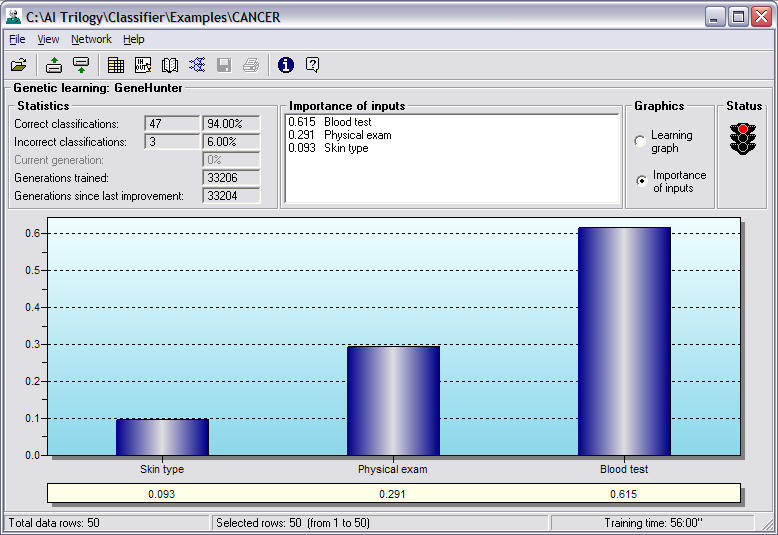
Importance of inputs: (Displayed when
you select the Importance of Inputs graph) Displays a list of
inputs and a corresponding number that indicates the importance
of the variable in correctly classifying the example. The higher
the number, the more important that variable is in classifying
the example.
The Relative Importance of Inputs graph
displays a bar chart of the input values based on the numbers
for each input displayed in the list described above. Click on
the right mouse button to either copy the list to the clipboard
for use in other Windows applications, save the list as a text
file which may be read by a word processor or spreadsheet, or
print the list.
If you switch to the Learning graph, the
following screen is displayed:
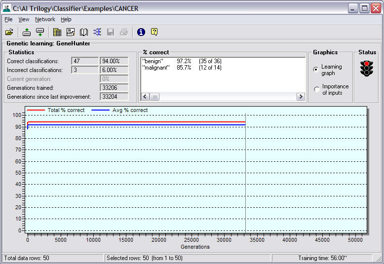
% Correct: (Displayed when you select
the Learning graph) Displays a list of available output
categories and the percentage of correct neural network classifications
based on examples in the training data.
The Correct Classifications by Generation
chart graphs: Total percent of correct classifications
predicted by the neural network over all classifications in the
training data. This number is computed by dividing the neural network's
total number of correct classifications for the training data by
the total number of examples in the training data. This is the
number optimized by the genetic algorithm when the Optimized of
% average checkbox is turned off in the Input/output selection
and training strategy selection screen in Step 8 of the
Instructor.
Average percent of correct classifications
predicted by the neural network for the training data. This number
is computed by adding the percent of correct classifications in
each output category for the training data and dividing that sum
by the number of output categories in the training data. This is
the number optimized by the genetic algorithm when the Optimized
of % average checkbox is turned on in the Input/output selection
and training strategy selection screen in Step 8 of the
Instructor.
Click on the right mouse button when the
pointer is inside the graph to display options to copy the graph
to the Windows clipboard for use in another document, to save
the graph as a bitmap file, or to print the graph.
Push the Next button to see the results.
Instructor Step 10 - Obtain Results (Genetic)
This screen displays the same
graphs and statistics shown for the neural training strategy. You will
notice that there are no significant differences between the neural and
genetic training strategies. This could change, however, depending upon
the problem and the number of training examples.
Write to a File
Once again you decide to save a
copy of the neural network’s classifications. Click on the Write to a File
button. A file is created which include
s the columns and rows from the
original file plus an additional column of neural network classifications. The
file is called CANCER.OUT as a default. The first part of the name
comes from the data file used to train the neural network, and the program adds
the .OUT extension. The file name may be changed in the dialog box.
Change the name to CANCERG.OUT
so you can compare results with the file called CANCER.OUT that was
previously trained with the Neural Training Strategy. This file is a
comma separated file that can be read by spreadsheets, notepads, and
word processors. The file is written in the same format (list
separator, decimal symbol
) as the input file format.
For quick reference, you click
on the Print Classifications button that prints out a report on the
default printer attached to your computer. The report include
s the row
number, an actual output value from the training data, and the
corresponding neural network classification for each row.

Push the Next button to jump to
Instructor Step 11.
Instructor Step 11 - Apply the Model to the Remaining Data Rows
(Genetic)
Since you trained the neural network
with all 50 rows of data, you can skip this step of the Instructor.
Push the Next button to jump to Instructor Step 12.
Instructor Step 12 - Save a Copy of the Neural Network (Genetic)
Use this step of the Instructor
to save a copy of the neural network on disk for later use. You may want to
apply this neural network later without taking the time to retrain it.
Save the neural network by pushing the Save
Net button. The neural network would ordinarily be saved under the default name of
CANCER.NET. Since, however, you already have a neural network trained with the
Neural Training Strategy with the name CANCER.NET, you should change the
name to CANCERG.NET.
The dialog box that is displayed gives you an option to change this
name. Record the file name and the fact that it was trained with the
Genetic Training Strategy.
Push the Next button to continue
with the Instructor.
Exit
Push the next button three
times to skip Steps 13, 14, and 15 because you have already retrained
the neural network. Instructor Step 16 allows you to close the Instructor by
clicking on the Exit button. You have finished training your models.
Examine the .OUT files in a spreadsheet program to see which model gave
better results.
